Difference between revisions of "Outputs"
(→DRGEP reaction) |
|||
| (27 intermediate revisions by the same user not shown) | |||
| Line 2: | Line 2: | ||
Once your "condition.cpp" is filled with the desired key words, you can run the code with | Once your "condition.cpp" is filled with the desired key words, you can run the code with | ||
| − | |||
| Line 13: | Line 12: | ||
and | and | ||
| − | + | ./mainProgram | |
| − | ./mainProgram | + | |
| − | + | ||
| + | just the first time. After, if you modify "input_file.ini" you can directly execute ./mainProgram with all the modifications taken into account. | ||
| + | |||
| + | Note that the Optimisation step of PremixedFlames and all the steps of the multipleInlet configuration (except getQSSfile) can be launched in parallel, for example on 8 proc, with : | ||
| + | |||
| + | mpirun -np 8 mainProgram | ||
If the main program is correctly running, your terminal should display the ORCh logo and all the information on your flame and your scheme. | If the main program is correctly running, your terminal should display the ORCh logo and all the information on your flame and your scheme. | ||
| − | The outputs depends on the step you are running | + | The outputs depends on the step you are running. |
| Line 27: | Line 29: | ||
== Compute Trajectories == | == Compute Trajectories == | ||
| − | This step | + | This step simply calculates the trajectories of the wanted mechanism. The .dat files are directly written in the output directory under the name "Premixed_.dat" for the 1D premixed configuration and under the name "Trajectory_X.dat" for the 0D stochastic configuration, with X the number of the inlets. |
== DRGEP species == | == DRGEP species == | ||
| Line 33: | Line 35: | ||
[[File:spec.png|300px|thumb|right|Exemple : List of the species with their interaction rate]] | [[File:spec.png|300px|thumb|right|Exemple : List of the species with their interaction rate]] | ||
| − | During this step, the main program will display every species of the scheme with the maximum of the interaction rates with the targeted species next to them. The interaction rates of targeted species are automatically set to 1. After that, new trajectories will be calculated with less and less species (until divergence with the reference trajectories), starting by the suppression of the less ranked ones. | + | During this step, the main program will display every species of the scheme with the maximum of the interaction rates with the targeted species next to them. The interaction rates of targeted species and the species into reactants are automatically set to 1. After that, new trajectories will be calculated with less and less species (until divergence with the reference trajectories), starting by the suppression of the less ranked ones. |
| − | Trajectories are then written in the repertory <code>/outputs</code> and new schemes in <code>/outputs/mechanisms</code>, with the name of the step | + | Trajectories are then written in the repertory <code>/outputs/Premixed</code> or <code>/outputs/Stochastic</code> and new schemes in <code>/outputs/mechanisms</code>, with the name of the step and the number of species. |
| − | + | Moreover, the interaction rates are saved in <code>DRGEP_Species.log</code>. | |
| + | |||
| + | Exemple : | ||
| + | |||
| + | For a 20 species reduced scheme for 1D premixed flames, the outputs are : | ||
| + | |||
| + | The mechanism : | ||
| + | outputs/mechanisms/drgepSpecies20.xml | ||
| + | |||
| + | The trajectory : | ||
| + | outputs/Premixed/Reduced_DRGEP_Species20_0.dat | ||
| + | |||
| + | And the trajectories of the species chosen by the user in "SpeciesToPlot" compared to the trajectory of the reference scheme : | ||
| + | outputs/Premixed/DRGEP_Species20_Flame0.dat | ||
== DRGEP reaction == | == DRGEP reaction == | ||
| Line 43: | Line 58: | ||
| − | [[File:reac.png|300px|thumb|right|Exemple : List of the | + | [[File:reac.png|300px|thumb|right|Exemple : List of the reactions with their interaction rate displayed during the run]] |
During this step, the main program will display every global, backwards and forwards reactions of the scheme with the maximum of the interaction rates with the targeted species next to them. After that, new trajectories will be calculated with less and less reactions (until divergence with the reference trajectories), starting by the suppression of the less ranked ones. | During this step, the main program will display every global, backwards and forwards reactions of the scheme with the maximum of the interaction rates with the targeted species next to them. After that, new trajectories will be calculated with less and less reactions (until divergence with the reference trajectories), starting by the suppression of the less ranked ones. | ||
| − | Trajectories are then written in the repertory <code>/outputs</code> | + | Trajectories are then written in the repertory <code>/outputs/Premixed</code> or <code>/outputs/Stochastic</code> and new schemes in <code>/outputs/mechanisms</code>, with the name of the step and the number of reactions. |
| − | + | Moreover, the interaction rates are saved in <code>DRGEP_Reactions.log</code>. | |
| + | |||
| + | Exemple : | ||
| + | |||
| + | For a 30 reactions reduced scheme for 0D stochastic configuration with 2 inlets, the outputs are : | ||
| + | |||
| + | The mechanism : | ||
| + | |||
| + | outputs/mechanisms/drgepReactions30.xml | ||
| + | |||
| + | The trajectories : | ||
| + | |||
| + | outputs/Stochastic/Reduced_DRGEP_Reactions30_0.dat | ||
| + | outputs/Stochastic/Reduced_DRGEP_Reactions30_1.dat | ||
| + | |||
| + | And the trajectories of the species chosen by the user in "SpeciesToPlot" compared to the trajectory of the reference scheme : | ||
| + | |||
| + | outputs/Stochastic/DRGEP_Reactions30_Inlet0.eps | ||
| + | outputs/Stochastic/DRGEP_Reactions30_Inlet1.eps | ||
== Compute QSS Criteria == | == Compute QSS Criteria == | ||
| + | [[File:computeQSSCriteria.png|300px|thumb|right|Example : QSS criteria]] | ||
| + | |||
| + | During this step, the main program displays the QSS criteria of each species and their interaction with the other. If this criteria is close to 0, the species is a good candidate to be in quasi steady state assumption. | ||
| + | |||
| + | A log file is also available at the end of this step. | ||
| + | |||
| + | Moreover, the species selected for QSS assumption must be in linear interaction with transported species. So if a species like CH3O in the screenshot example is put to QSS assumption, all the species linked to CH3O like OH, O and H cannot be put in QSS assumption, even if their QSS criteria is low. | ||
| + | |||
| + | This step does not generate outputs, it is just a tool to determine which species can be put in QSS assumption. | ||
== Get QSS file == | == Get QSS file == | ||
| − | + | This step generates the analytic scheme trajectories with the list of the QSS species. The user can choose to test N lists of QSS species, and all the outputs will be placed in the following directories : | |
| + | analytic_schemes/RefQSSAnalysis0/ | ||
| + | analytic_schemes/RefQSSAnalysis1/ | ||
| + | ... | ||
| + | analytic_schemes/RefQSSAnalysisN-1/ | ||
| + | |||
| + | |||
| + | In each RefQSSAnalysis/ directory, the trajectories and the associated plots are written. | ||
| + | |||
| + | Example : If 2 species are put in QSS assumption from a 14 species scheme, the outputs are : | ||
| + | |||
| + | the trajectory : | ||
| + | |||
| + | <code> Reduced_QSS12_0.dat</code> | ||
| + | |||
| + | The trajectory plots against the reference scheme : | ||
| + | |||
| + | <code>QSS12_Flame0.eps</code> | ||
| + | |||
| + | |||
| + | Nota bene : The fitness displayed in the graphs is the one between the current reduced trajectories and the trajectories of the reference scheme chosen by the user. | ||
== Optimisation == | == Optimisation == | ||
| + | This step generates N elements of a population of analytic schemes at each generation with different Arrhenius factors. It is recommended to divide the elements on several processes in order to have a population as large as possible. | ||
| + | |||
| + | A log file is available during the optimisation step with all the fitnesses at each generation. | ||
| + | |||
| + | The outputs of interest are all placed in the following directory : | ||
| + | |||
| + | analytic_schemes/PLOTS | ||
| + | |||
| + | where the evolution of the best scheme fitness is plotted at each generation along with the plots of the trajectories of the best scheme. This step ends when all the generations have run, but with these outputs the user can choose to end this step sooner. | ||
| + | |||
| + | Example : | ||
| + | |||
| + | Trajectory plot of the best scheme at the third generation written in : | ||
| + | analytic_schemes/PLOTS/GEN3_POP0_FIT-1096_Flame0.eps | ||
| + | |||
| + | and the N analytic schemes divided on the p processes are calculated on the Ref files : | ||
| + | |||
| + | analytic_schemes/Ref0 | ||
| + | analytic_schemes/Ref1 | ||
| + | ... | ||
| + | analytic_schemes/Refp-1 | ||
| + | |||
| + | |||
| + | Finally the best scheme at each generation is placed in the directory : | ||
| − | + | analytic_schemes/Ref/ | |
Latest revision as of 15:34, 1 February 2019
Once your "condition.cpp" is filled with the desired key words, you can run the code with
make clean
make
and
./mainProgram
just the first time. After, if you modify "input_file.ini" you can directly execute ./mainProgram with all the modifications taken into account.
Note that the Optimisation step of PremixedFlames and all the steps of the multipleInlet configuration (except getQSSfile) can be launched in parallel, for example on 8 proc, with :
mpirun -np 8 mainProgram
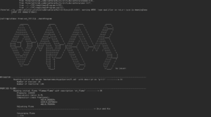
If the main program is correctly running, your terminal should display the ORCh logo and all the information on your flame and your scheme.
The outputs depends on the step you are running.
Contents
Compute Trajectories
This step simply calculates the trajectories of the wanted mechanism. The .dat files are directly written in the output directory under the name "Premixed_.dat" for the 1D premixed configuration and under the name "Trajectory_X.dat" for the 0D stochastic configuration, with X the number of the inlets.
DRGEP species
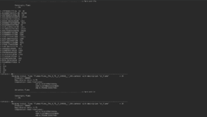
During this step, the main program will display every species of the scheme with the maximum of the interaction rates with the targeted species next to them. The interaction rates of targeted species and the species into reactants are automatically set to 1. After that, new trajectories will be calculated with less and less species (until divergence with the reference trajectories), starting by the suppression of the less ranked ones.
Trajectories are then written in the repertory /outputs/Premixed or /outputs/Stochastic and new schemes in /outputs/mechanisms, with the name of the step and the number of species.
Moreover, the interaction rates are saved in DRGEP_Species.log.
Exemple :
For a 20 species reduced scheme for 1D premixed flames, the outputs are :
The mechanism :
outputs/mechanisms/drgepSpecies20.xml
The trajectory :
outputs/Premixed/Reduced_DRGEP_Species20_0.dat
And the trajectories of the species chosen by the user in "SpeciesToPlot" compared to the trajectory of the reference scheme :
outputs/Premixed/DRGEP_Species20_Flame0.dat
DRGEP reaction
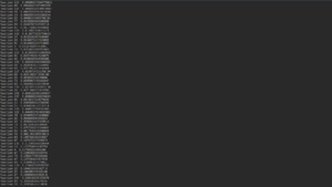
During this step, the main program will display every global, backwards and forwards reactions of the scheme with the maximum of the interaction rates with the targeted species next to them. After that, new trajectories will be calculated with less and less reactions (until divergence with the reference trajectories), starting by the suppression of the less ranked ones.
Trajectories are then written in the repertory /outputs/Premixed or /outputs/Stochastic and new schemes in /outputs/mechanisms, with the name of the step and the number of reactions.
Moreover, the interaction rates are saved in DRGEP_Reactions.log.
Exemple :
For a 30 reactions reduced scheme for 0D stochastic configuration with 2 inlets, the outputs are :
The mechanism :
outputs/mechanisms/drgepReactions30.xml
The trajectories :
outputs/Stochastic/Reduced_DRGEP_Reactions30_0.dat
outputs/Stochastic/Reduced_DRGEP_Reactions30_1.dat
And the trajectories of the species chosen by the user in "SpeciesToPlot" compared to the trajectory of the reference scheme :
outputs/Stochastic/DRGEP_Reactions30_Inlet0.eps
outputs/Stochastic/DRGEP_Reactions30_Inlet1.eps
Compute QSS Criteria
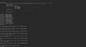
During this step, the main program displays the QSS criteria of each species and their interaction with the other. If this criteria is close to 0, the species is a good candidate to be in quasi steady state assumption.
A log file is also available at the end of this step.
Moreover, the species selected for QSS assumption must be in linear interaction with transported species. So if a species like CH3O in the screenshot example is put to QSS assumption, all the species linked to CH3O like OH, O and H cannot be put in QSS assumption, even if their QSS criteria is low.
This step does not generate outputs, it is just a tool to determine which species can be put in QSS assumption.
Get QSS file
This step generates the analytic scheme trajectories with the list of the QSS species. The user can choose to test N lists of QSS species, and all the outputs will be placed in the following directories :
analytic_schemes/RefQSSAnalysis0/
analytic_schemes/RefQSSAnalysis1/
...
analytic_schemes/RefQSSAnalysisN-1/
In each RefQSSAnalysis/ directory, the trajectories and the associated plots are written.
Example : If 2 species are put in QSS assumption from a 14 species scheme, the outputs are :
the trajectory :
Reduced_QSS12_0.dat
The trajectory plots against the reference scheme :
QSS12_Flame0.eps
Nota bene : The fitness displayed in the graphs is the one between the current reduced trajectories and the trajectories of the reference scheme chosen by the user.
Optimisation
This step generates N elements of a population of analytic schemes at each generation with different Arrhenius factors. It is recommended to divide the elements on several processes in order to have a population as large as possible.
A log file is available during the optimisation step with all the fitnesses at each generation.
The outputs of interest are all placed in the following directory :
analytic_schemes/PLOTS
where the evolution of the best scheme fitness is plotted at each generation along with the plots of the trajectories of the best scheme. This step ends when all the generations have run, but with these outputs the user can choose to end this step sooner.
Example :
Trajectory plot of the best scheme at the third generation written in :
analytic_schemes/PLOTS/GEN3_POP0_FIT-1096_Flame0.eps
and the N analytic schemes divided on the p processes are calculated on the Ref files :
analytic_schemes/Ref0
analytic_schemes/Ref1
...
 analytic_schemes/Refp-1
Finally the best scheme at each generation is placed in the directory :
analytic_schemes/Ref/


